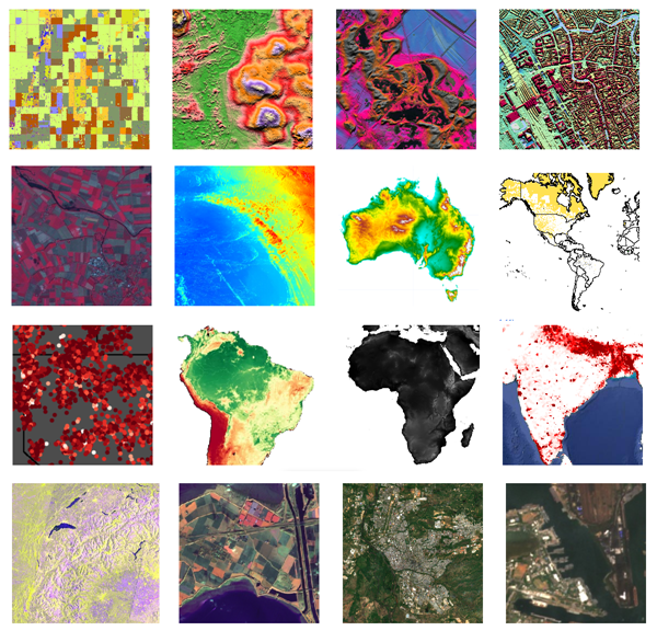
Google Earth Engine provides cloud-computing platform for Remote Sensing analysis. There are many datasets available. The following images are mostly used images.
- Landsat 8
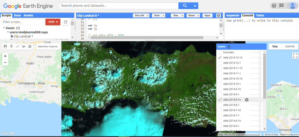
Landsat 8 is multi-spectral image. Check how to make image composite here. The script below will show the collection of Landsat 8 image in the whole year of 2014. Landsat 8 is available starting from February 2013.
// Composite an image collection and clip it to a boundary.

var i;
var j;

// set date 2015 - 2019
var tahun = [2014];
var bulan = [1,1,2,2,3,3,  4,4,5,5,6,6,  7,7,8,8,9,9,  10,10,11,11,12,12];
var tgl1 = [1,16,1,16,1,16,  1,16,1,16,1,16,  1,16,1,16,1,16,  1,16,1,16,1,16];
var tgl2 = [15,31,15,28,15,31,  15,30,15,31,15,30,  15,31,15,31,15,30,  15,31,15,30,15,31];


// Load every Landsat 8 raw imagery in 2014.
for (i = 0; i<tahun.length;i++){
  for(j = 0; j<bulan.length;j++){
    var composite = ee.ImageCollection('LANDSAT/LC08/C01/T1_TOA')
    .filterDate( tahun[i] + "-" + bulan[j]  + "-" + tgl1[j], tahun[i] + "-" + bulan[j] + "-" + tgl2[j])
    .median();

    // Clip to the output image to the geometry boundary.
    var clipped = composite.clip(geometry);

    Map.addLayer(clipped , {bands: ['B6', 'B5', 'B4']}, "date " + tahun[i] + "-" + bulan[j]  + "-" + tgl1[j], false );
  }
}


// Display the result.
Map.setCenter(113.517, -8.1631, 9);
Map.addLayer(clipped, {color: 'FFFFFF'}, 'boundary', false);
//print('Polygon area: ', geometry.area().divide(100 * 100));


// Export the FeatureCollection to a SHP file.
Export.table.toDrive({
  collection: clipped,
  description:'Mount Bromo',
  fileFormat: 'SHP'
});
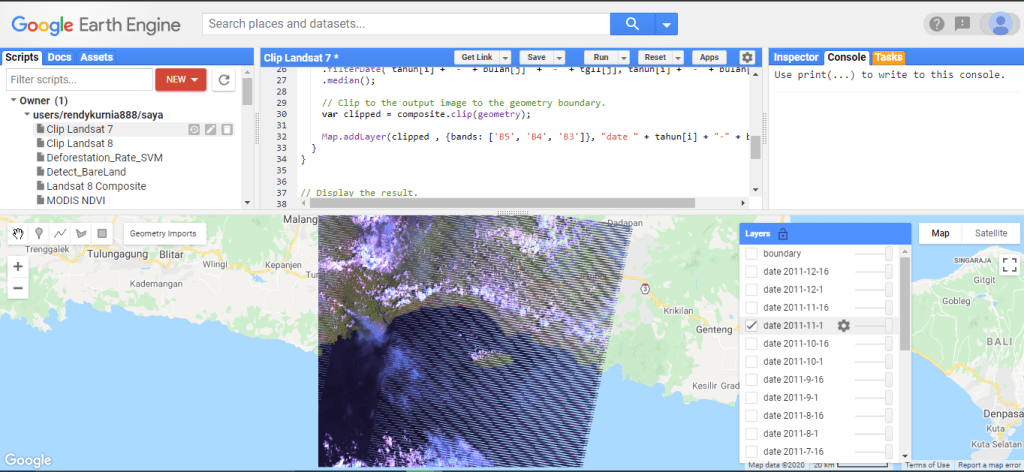
- Landsat 7.
Landsat 7 was launched in April 1999. The script below show Landsat images for the 1 hole year. The latest Landsat 7 images have interrupting black stripes.
// Composite an image collection and clip it to a boundary.

var i;
var j;

// set year 2011
var tahun = [2011];
var bulan = [1,1,2,2,3,3,  4,4,5,5,6,6,  7,7,8,8,9,9,  10,10,11,11,12,12];
var tgl1 = [1,16,1,16,1,16,  1,16,1,16,1,16,  1,16,1,16,1,16,  1,16,1,16,1,16];
var tgl2 = [15,31,15,28,15,31,  15,30,15,31,15,30,  15,31,15,31,15,30,  15,31,15,30,15,31];


// Load every Landsat 7 raw imagery in 2011.
for (i = 0; i<tahun.length;i++){
  for(j = 0; j<bulan.length;j++){
    var composite = ee.ImageCollection('LANDSAT/LE07/C01/T1')
    .filterDate( tahun[i] + "-" + bulan[j]  + "-" + tgl1[j], tahun[i] + "-" + bulan[j] + "-" + tgl2[j])
    .median();

    // Clip to the output image to the geometry boundary.
    var clipped = composite.clip(geometry);

    Map.addLayer(clipped , {bands: ['B5', 'B4', 'B3']}, "date " + tahun[i] + "-" + bulan[j]  + "-" + tgl1[j], false );
  }
}


// Display the result.
Map.setCenter(113.517, -8.1631, 9);
Map.addLayer(clipped, {color: 'FFFFFF'}, 'boundary', false);


// Export the FeatureCollection to a SHP file.
Export.table.toDrive({
  collection: clipped,
  description:'Mount Bromo',
  fileFormat: 'SHP'
});
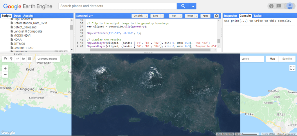
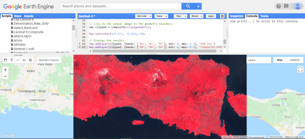
3. Sentinel-2
The script here shows Sentinel-2 image in 2020 with cloud mask.
// This example uses the Sentinel-2 QA band to cloud mask
// the collection.  The Sentinel-2 cloud flags are less
// selective, so the collection is also pre-filtered by the
// CLOUDY_PIXEL_PERCENTAGE flag, to use only relatively
// cloud-free granule.

// Function to mask clouds using the Sentinel-2 QA band.
function maskS2clouds(image) {
  var qa = image.select('QA60')

  // Bits 10 and 11 are clouds and cirrus, respectively.
  var cloudBitMask = 1 << 10;
  var cirrusBitMask = 1 << 11;

  // Both flags should be set to zero, indicating clear conditions.
  var mask = qa.bitwiseAnd(cloudBitMask).eq(0).and(
             qa.bitwiseAnd(cirrusBitMask).eq(0))

  // Return the masked and scaled data, without the QA bands.
  return image.updateMask(mask).divide(10000)
      .select("B.*")
      .copyProperties(image, ["system:time_start"])
}

// Map the function over one year of data and take the median.
// Load Sentinel-2 TOA reflectance data.
var collection = ee.ImageCollection('COPERNICUS/S2')
    .filterDate('2020-01-01', '2020-7-31')
    // Pre-filter to get less cloudy granules.
    .filter(ee.Filter.lt('CLOUDY_PIXEL_PERCENTAGE', 20))
    .map(maskS2clouds)

var composite = collection.median()

// Clip to the output image to the geometry boundary.
var clipped = composite.clip(geometry);

Map.setCenter(113.517, -8.1631, 9);

// Display the results.
Map.addLayer(clipped, {bands: ['B4', 'B3', 'B2'], min: 0, max: 0.3}, 'RGB 432')
Map.addLayer(clipped, {bands: ['B8', 'B4', 'B3'], min: 0, max: 0.3}, 'Composite 843')
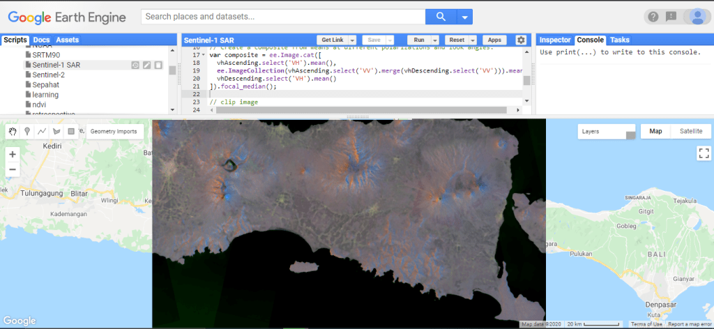
4. Sentinel-1 SAR
// Load the Sentinel-1 ImageCollection.
var sentinel1 = ee.ImageCollection('COPERNICUS/S1_GRD');

// Filter by metadata properties.
var vh = sentinel1
  // Filter to get images with VV and VH dual polarization.
  .filter(ee.Filter.listContains('transmitterReceiverPolarisation', 'VV'))
  .filter(ee.Filter.listContains('transmitterReceiverPolarisation', 'VH'))
  // Filter to get images collected in interferometric wide swath mode.
  .filter(ee.Filter.eq('instrumentMode', 'IW'));

// Filter to get images from different look angles.
var vhAscending = vh.filter(ee.Filter.eq('orbitProperties_pass', 'ASCENDING'));
var vhDescending = vh.filter(ee.Filter.eq('orbitProperties_pass', 'DESCENDING'));

// Create a composite from means at different polarizations and look angles.
var composite = ee.Image.cat([
  vhAscending.select('VH').mean(),
  ee.ImageCollection(vhAscending.select('VV').merge(vhDescending.select('VV'))).mean(),
  vhDescending.select('VH').mean()
]).focal_median();

// clip image
var clipped = composite.clip(geometry);

// Display as a composite of polarization and backscattering characteristics.
Map.setCenter(113.517, -8.1631, 9);
Map.addLayer(clipped, {min: [-25, -20, -25], max: [0, 10, 0]}, 'local');
Map.addLayer(composite, {min: [-25, -20, -25], max: [0, 10, 0]}, 'global', false);
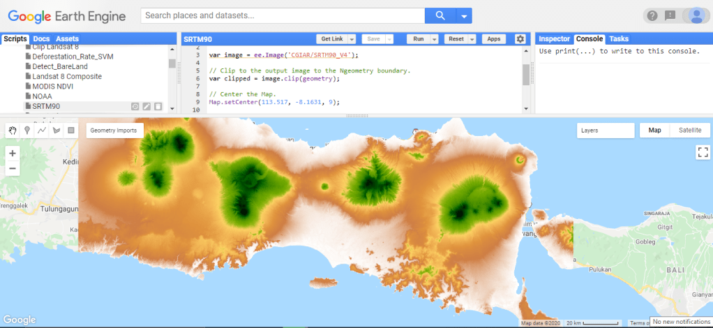
5. SRTM (Shuttle Radar Topography Mission)
SRTM shows Digital Surface Model (DSM) in color grading. High altitude to lo altitude is represented in colors from green, yelloe, orange, and red.
// Display SRTM image.

var image = ee.Image('CGIAR/SRTM90_V4');

// Clip to the output image to the geometry boundary.
var clipped = image.clip(geometry);

// Center the Map.
Map.setCenter(113.517, -8.1631, 9);

// Make a palette: a list of hex strings.
var palette = ['FFFFFF', 'CE7E45', 'DF923D', 'F1B555', 'FCD163', '99B718',
               '74A901', '66A000', '529400', '3E8601', '207401', '056201',
               '004C00', '023B01', '012E01', '011D01', '011301'];

// Display the image.
Map.addLayer(clipped, {min: 0, max: 3000, palette:palette}, 'SRTM');
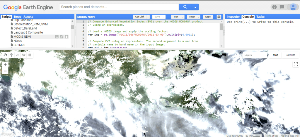
6. MODIS (Moderate Resolution Imaging Spectroradiometer)
// Compute Enhanced Vegetation Index (EVI) over the MODIS MOD09GA product
// using an expression.

// Load a MODIS image and apply the scaling factor.
var img = ee.Image('MODIS/006/MOD09GA/2012_03_09').multiply(0.0001);

// Compute EVI using an expression.  The second argument is a map from
// variable name to band name in the input image.
var evi = img.expression(
    '2.5 * (nir - red) / (nir + 6 * red - 7.5 * blue + 1)',
    {
        red: img.select('sur_refl_b01'),    // 620-670nm, RED
        nir: img.select('sur_refl_b02'),    // 841-876nm, NIR
        blue: img.select('sur_refl_b03')    // 459-479nm, BLUE
    });


// Center the map.
Map.setCenter(113.517, -8.1631, 9);

// Display the input image and the EVI computed from it.
Map.addLayer(img.select(['sur_refl_b01', 'sur_refl_b04', 'sur_refl_b03']),
         {min: 0, max: 0.2}, 'MODIS bands 1/4/3');
Map.addLayer(evi, {min: 0, max: 1}, 'EVI');
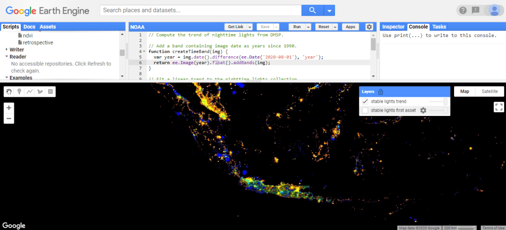
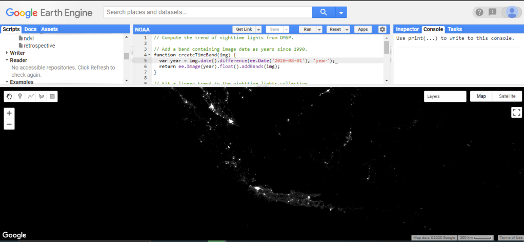
7. NOAA (National Oceanic and Atmospheric Administration)
// Compute the trend of nighttime lights from DMSP.

// Add a band containing image date as years since 1990.
function createTimeBand(img) {
  var year = img.date().difference(ee.Date('2020-08-01'), 'year');
  return ee.Image(year).float().addBands(img);
}

// Fit a linear trend to the nighttime lights collection.
var collection = ee.ImageCollection('NOAA/DMSP-OLS/CALIBRATED_LIGHTS_V4')
    .select('avg_vis')
    .map(createTimeBand);
var fit = collection.reduce(ee.Reducer.linearFit());

// Display a single image
Map.addLayer(ee.Image(collection.select('avg_vis').first()),
         {min: 0, max: 63},
         'stable lights first asset');

// Display trend in red/blue, brightness in green.
Map.setCenter(107.404, -3.463, 5);
Map.addLayer(fit,
         {min: 0, max: [0.18, 20, -0.18], bands: ['scale', 'offset', 'scale']},
         'stable lights trend');