

This one article discusses two Machine Learning methods. They are Decision Tree (also known as Classification and Regression Tree) and later Random Forest. Decision tree, as its name suggests, takes the form of tree to decide which classification new observations are in. Mostly, we actually have used this decision tree method in daily life to decide things. If A happens, then do B. Or else, do C. This Decision Tree in Machine Learning will build a Decision Tree according to the data user feeds to the model. If you are not familiar with Machine Learning basic, please find an article discussing it here. After that, come back here to this article again.
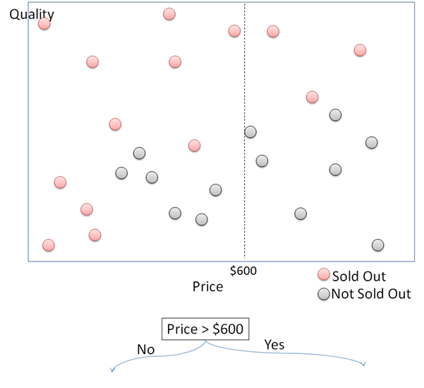
How Decision Tree works in simple way is expressed using the following data. This plot shows purchased goods plotted for their price in x axis and quality in y axis. The purchased goods are then divided into “sold out” and “not sold out”. This article will try to build a Decision Tree to detect whether a thing will be sold out or not according to its price and quality.

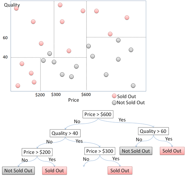
First, split the data points into two divisions by the price. Data points with price higher and lower than $600 are divided into right and left. For each of the side, split the data points again into 2 parts according to the quality. For data points with price above $600, they will be sold out if the quality is above 60, and not sold out if the quality is under 60. This process continues to divide those data points while growing the Decision Tree.


The example above illustrate growing Decision Tree in simple way as the data points only have 2 dimensions. Things will be more complicated if the data has more than 3 dimensions or parameters. To practice this, we will use Hotel Customer Data. The data is dummy data I created. The data contains the information of customers opinion of a hotel. There are 500 observations or rows in this data frame. Each observation represents one customer. There are 12 variables, with data structure as following.
>str(CustomerData)
data.frame':	500 obs. of  12 variables:
 $ Id          : int  1 2 3 4 5 6 7 8 9 10 ...
 $ Gender      : Factor w/ 2 levels "Female","Male": 1 1 1 2 2 2 2 1 2 2 ...
 $ Age         : num  33 30 37 34 33 34 35 30 39 34 ...
 $ Purpose     : Factor w/ 2 levels "Business","Personal": 2 2 2 2 2 2 2 2 1 2 ...
 $ RoomType    : Factor w/ 3 levels "Double","Family",..: 1 2 3 1 1 1 1 2 1 1 ...
 $ Food        : num  21 32 46 72 84 67 56 10 73 97 ...
 $ Bed         : num  53 32 25 30 7 46 0 19 12 30 ...
 $ Bathroom    : num  24 18 29 15 43 16 0 1 62 26 ...
 $ Cleanness   : num  44 44 20 55 78 61 9 53 65 59 ...
 $ Service     : num  46 74 24 38 51 44 32 58 56 46 ...
 $ Satisfaction: Factor w/ 3 levels "Dissatisfied",..: 1 1 1 1 2 2 1 1 2 2 ...
 $ Repeat      : Factor w/ 2 levels "No","Repeat": 2 1 1 2 2 1 1 2 2 1 ...

Customers are requested to fill a survey form to score 5 parameters of the hotel and finally give an overall satisfaction conclusion. The 5 parameters are food, bed, bathroom, cleanness, and service. The five parameters are scored in numeric from 0 to 100. 0 represents very bad and 100 represents very good. The overall satisfaction asks the customer to fill one from three classes, satisfied, neutral, or dissatisfied. There are other variables, like age, purpose, room type, and repeat, but they are not discussed in this article.

The script below will grow a Decision Tree using 3 parameters of hotel customers: gender, purpose, and room type to classify customers overall satisfaction. The three parameters are in categorical format. The satisfaction classification is expressed in 3 classes. They are “satisfied”, “neutral”, and “dissatisfied”.
# Load the rpart package
library(rpart)

# Build a model to predict according to selected parameters. Here we try categorical parameters
TreeModel <- rpart(Satisfaction~Gender+ Purpose + RoomType, data = trainCustomer, method = "class", control = rpart.control(cp = 0))

# predict the test data
predictTree <- predict(TreeModel, testCustomer, type = "class")

# Load the rpart.plot package
library(rpart.plot)

# visualize the decision tree
rpart.plot(TreeModel, tweak = 1.5)

> # percentage of accuracy
> table(predictTree, testCustomer$Satisfaction)

predictTree    Dissatisfied Neutral Satisfied
  Dissatisfied           16      16         8
  Neutral                15      24        21
  Satisfied               0       0         0
> mean(predictTree == testCustomer$Satisfaction)
[1] 0.4
The accuracy is very low, only 40%. Now, the Decision Tree script will be run again. This time all of the parameters or predictors will be used. The model later will decided itself which parameters are most significant to grow the Decision Tree. It even cannot predict “Satisfied”.
# Create decision tree model using all of the parameters
TreeModel2 <- rpart(Satisfaction ~ ., data = trainCustomer, method = "class", control = rpart.control(cp = 0))

# predict the test data
predictTree2 <- predict(TreeModel2, testCustomer, type = "class")

# visualize the decision tree
rpart.plot(TreeModel2, tweak = 1.3)

head(data.frame(testCustomer[,c(6:9, 11)],predictTree2), 20)
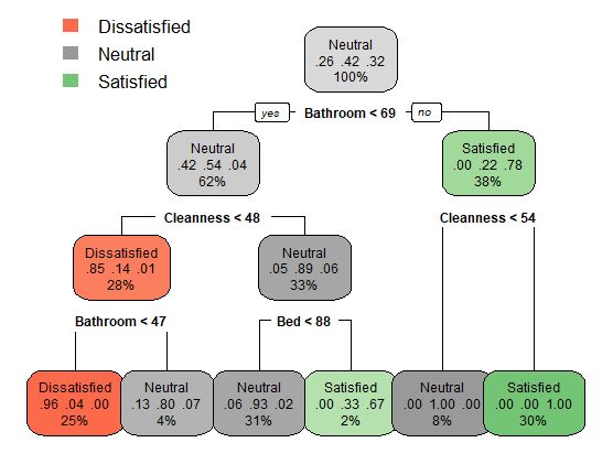
The second Decision Tree here has high accuracy of 89% in classifying the customer overall satisfaction. It takes “bathroom”, “cleanness, “bed”, and “food” s its predictors. Find the generated Decision Tree below.

> # percentage of accuracy
> mean(predictTree2 == testCustomer$Satisfaction)
[1] 0.89
> table(predictTree2, testCustomer$Satisfaction)

predictTree2   Dissatisfied Neutral Satisfied
  Dissatisfied           26       4         0
  Neutral                 4      36         2
  Satisfied               1       0        27
Here is the classification result of the first 20 observations of the test data.
    Food Bed Bathroom Cleanness Satisfaction predictTree2
488   42  64       68        40      Neutral      Neutral
158  100  37       25        59      Neutral      Neutral
126   55  80       93        84    Satisfied    Satisfied
113  100  87       63        72    Satisfied      Neutral
325   58  32        0        19 Dissatisfied Dissatisfied
421   82 100       70        83    Satisfied    Satisfied
154   82  45       10        99      Neutral      Neutral
481   92  89       86       100    Satisfied    Satisfied
253   15  70       38         0 Dissatisfied Dissatisfied
460   28  51       84        20      Neutral      Neutral
64    23  33       29        86      Neutral Dissatisfied
373   51  69       53        78      Neutral      Neutral
89    67  46       16        61      Neutral      Neutral
402   25  36       11        23 Dissatisfied Dissatisfied
252   42  60       90        12      Neutral      Neutral
406   45  40       14        32 Dissatisfied Dissatisfied
67    83  61       15        79      Neutral      Neutral
128   89  86      100       100    Satisfied    Satisfied
280   94  52       90        72    Satisfied    Satisfied
392   34  38        5         8 Dissatisfied Dissatisfied
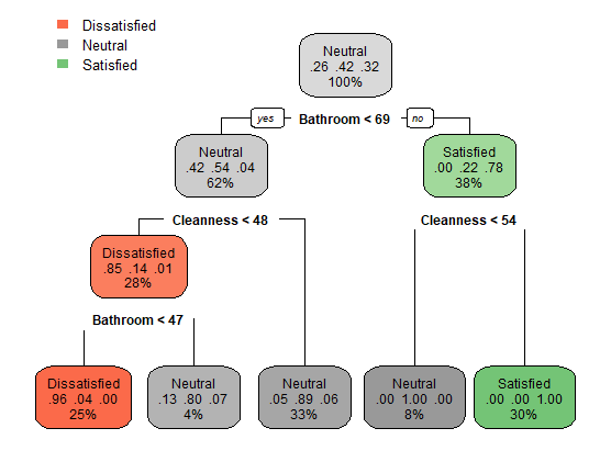
The created Decision Tree above has depth of 4. Now, examine the script below that build another Decision Tree model using the argument maxdepth = 3. This limits the maximum depth of the Decision Tree to be 3. We can see that by cutting the overgrown branch can actually increase the accuracy. The accuracy of the third Decision Tree we have is 91%. The Decision Tree now is also more simple than the previous one.
# Tend to of overgrown tree
# set the maxdepth of 3 for the tree
TreeModel3 <- rpart(Satisfaction ~ ., data = trainCustomer, method = "class", control = rpart.control(cp = 0, maxdepth = 3))

# Predict the test data
predictTree3 <- predict(TreeModel3, testCustomer, type = "class")

# plot the decision tree
rpart.plot(TreeModel3,  tweak = 1.3)
> # Compute the accuracy of the simpler tree
> mean(predictTree3 == testCustomer$Satisfaction)
[1] 0.91
> table(predictTree3, testCustomer$Satisfaction)

predictTree3   Dissatisfied Neutral Satisfied
  Dissatisfied           25       1         0
  Neutral                 5      39         2
  Satisfied               1       0        27
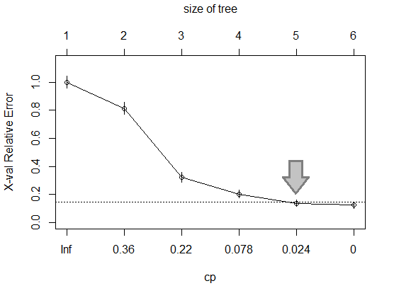
Another way to make the Decision Tree to be more simple is pruning. After the Decision Tree is grown, it can be seen as too complicated. Pruning can be applied to reduce less important branches of the Decision Tree so that it is less complicated. Cutting the less important branches is done at the least complex point where relative error does not decrease significantly anymore. The plot below shows the relative error in y-axis and cp in x-axis representing the complexity. The relative error drops when The Decision Tree gets more complex, or cp approaches 0. Figure out that c = 0.024 is the point where relative error does not decrease significantly anymore if the the cp is reduced.
# Examine the complexity plot
plotcp(TreeModel3)
# Prune the tree
TreeModel3_pruned <- prune(TreeModel3, cp = 0.024 )

rpart.plot(TreeModel3_pruned)

# Predict the test data
predictTree3_pruned <- predict(TreeModel3_pruned, testCustomer, type = "class")
Here is the result and accuracy of the Decision Tree model after pruned with cp = 0.024.
> mean(predictTree3_pruned == testCustomer$Satisfaction)
[1] 0.9
> table(predictTree3_pruned, testCustomer$Satisfaction)

predictTree3_pruned Dissatisfied Neutral Satisfied
       Dissatisfied           25       1         0
       Neutral                 6      39         3
       Satisfied               0       0        26
Now, we will discuss another Machine Learning method which still related to the Decision Tree. It is called Random Forest. The Random Forest model creates a number of different Decision Trees using the same data. When the test data are input into the Random Forest model, all of the Decision Trees will classify the test data. After that, the Decision Trees will vote which classification the test data are in.
The picture below illustrates Random Forest which is composed of a number of Decision Trees. Each Decision Tree classifies test data into class “A” and “B”. Since there are more Decision Trees that classifies the test data into “A”, it is decided that the test data is classified into “A” class.

The script below tries to classify the hotel customer satisfaction using Random Forest method.
> mean(PredictRF == testCustomer$Satisfaction)
[1] 0.97
> table(PredictRF, testCustomer$Satisfaction)

PredictRF      Dissatisfied Neutral Satisfied
  Dissatisfied           29       0         0
  Neutral                 2      40         1
  Satisfied               0       0        28

2 thoughts on “Decision Tree/Classification and Regression Tree and Random Forest”