

kNN is a supervised machine learning that detects the class of a new observation according to the distance to the other nearest neighboring training data. The k defines the number of nearest neighbors or training data point to use to classify the observation. This article discussion assumes that we have understood basic Machine Learning. If not, please go to this article, discussing about Machine Learning basic, and then come back here again.
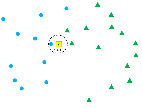
The figure below shows an illustration of how kNN works in classifying a new observation data according to existing training data. Yellow square with a question mark inside represents new observation that we want to classify. Blue circles and green triangles are labeled training data. They are located in 2-dimension diagram illustrating a set of training data with 2 parameters and classifications, blue circle and green triangle.

As mentioned earlier, the yellow square will be classified into blue circle or green circle according to its nearest neighboring training data. If we set k = 1, the yellow square will be classified into blue circle group because the most nearest training data point is the blue circle.
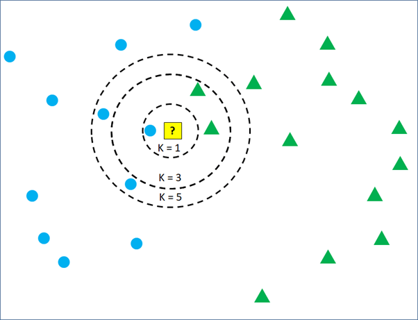
But, if k = 3 is set, the classification will take into account the 3 nearest training data point. In Figure 3, we can see that there are 2 green triangles and 1 blue circle being the closest to the new observation. Then, the new observation will be classified as green triangles. Changing the number of k from 1 to 3 can change the classification result.

Again, set the k = 5 and the yellow square will be classified into blue circle again because there are more blue circles than green triangles in the 5 nearest training data point. Now, what will the yellow square classified into, if the k is set to be 10?

It is still easy to do the classification because the example data above are visualized in 2 dimensions. Three dimensions data also still can be visualized. But, things will get more complicated if the data have more than 3 dimensions and many classifications. kNN algorithm plays a very important role to do the job.
Now, let’s try to do kNN classification using other data. Which data are we going to use for kNN? Is it the legendary iris data provided as built-in dataset. There are already many online posts and tutorials using iris data for various kinds of analysis, including Machine Learning and kNN. But, I have searched other all built-in data and can not find more suitable data to perform kNN. Okay, I will use “Hotel Customer data”. The data is dummy data I created. The data contains the information of customers opinion of a hotel. There are 500 observations or rows in this data frame. Each observation represents one customer. There are 12 variables, with data structure as following.
>str(CustomerData)
data.frame':	500 obs. of  12 variables:
 $ Id          : int  1 2 3 4 5 6 7 8 9 10 ...
 $ Gender      : Factor w/ 2 levels "Female","Male": 1 1 1 2 2 2 2 1 2 2 ...
 $ Age         : num  33 30 37 34 33 34 35 30 39 34 ...
 $ Purpose     : Factor w/ 2 levels "Business","Personal": 2 2 2 2 2 2 2 2 1 2 ...
 $ RoomType    : Factor w/ 3 levels "Double","Family",..: 1 2 3 1 1 1 1 2 1 1 ...
 $ Food        : num  21 32 46 72 84 67 56 10 73 97 ...
 $ Bed         : num  53 32 25 30 7 46 0 19 12 30 ...
 $ Bathroom    : num  24 18 29 15 43 16 0 1 62 26 ...
 $ Cleanness   : num  44 44 20 55 78 61 9 53 65 59 ...
 $ Service     : num  46 74 24 38 51 44 32 58 56 46 ...
 $ Satisfaction: Factor w/ 3 levels "Dissatisfied",..: 1 1 1 1 2 2 1 1 2 2 ...
 $ Repeat      : Factor w/ 2 levels "No","Repeat": 2 1 1 2 2 1 1 2 2 1 ...
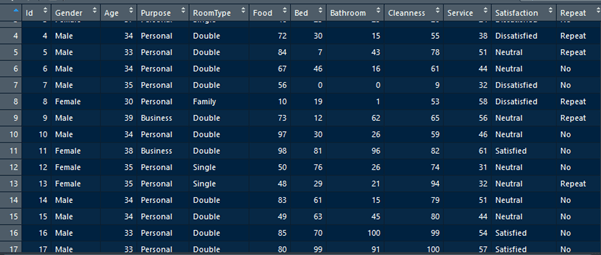
Customers are requested to fill a survey form to score 5 parameters of the hotel and finally give an overall satisfaction conclusion. The 5 parameters are food, bed, bathroom, cleanness, and service. The five parameters are scored in numeric from 0 to 100. 0 represents very bad and 100 represents very good. The overall satisfaction asks the customer to fill one from three classes, satisfied, neutral, or dissatisfied. There are other variables, like age, purpose, room type, and repeat, but they are not discussed in this article.
The goal of this article is to build a classification model to identify customer satisfaction class according to the 5 numeric parameters. Before that, let’s visualize the data distribution of each parameter by the satisfaction class.
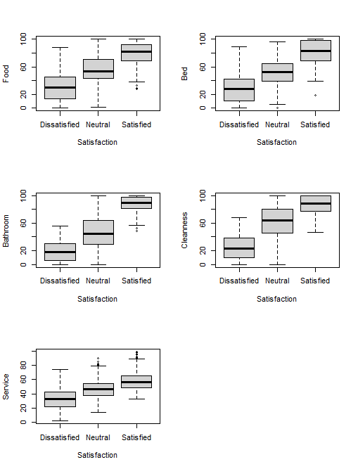
The figure below plots parameters of bed and food in to dimension. We can clearly see how satisfaction classes are determined by the two parameters. In the another figure, parameters are plotted in 3 dimensions scatter plot. But, the customer dataset has 5 parameters, so it cannot be plotted completely.
ggplot(CustomerData, aes(x =Food, y = Bed, col = Satisfaction))+geom_point(alpha=0.5)

shapes <- c(18,17,16)
shapes <- shapes[as.numeric(CustomerData$Satisfaction)]
colors <- c("red","green","blue")
colors <- colors[as.numeric(CustomerData$Satisfaction)]

plot3d <- scatterplot3d(CustomerData[,6:8], pch=shapes, color=colors)

From the 500 observations in the dataset, 20% will be sampled randomly to make the test data. The remaining 80% will become the training data. The training data are fed to the kNN to study the pattern. After that, the kNN model will detect the classification of the test data. The percentage of accuracy will be calculated according to the result of classifying the test data.
# Machine Learning
# create 100 test data from CustomerData, 20% of the  total data
sample_customer <- sample(500, 100, replace = FALSE)

#create test data
testCustomer <- CustomerData[sample_customer,]

# create 400 train data after excluding the 100 test data
trainCustomer <- CustomerData[-sample_customer,]

# Load the 'class' package
library(class)

# Create labels from train data
labelSatisfaction <- trainCustomer$Satisfaction

# Classify test data using kNN
predictkNN_customer <- knn(train = trainCustomer[c(6:10)], test = testCustomer[c(6:10)], cl = labelSatisfaction)
This matrix shows how many classifications are made correctly by the model and how many are mistaken for another model. The accuracy is 91%. From 100 test data, the kNN model detects correctly 91 observations.
> # accuracy
> # Create matrix to see predicted result and actual
> table(predictkNN_customer, testCustomer$Satisfaction)

predictkNN_customer Dissatisfied Neutral Satisfied
       Dissatisfied           24       1         0
       Neutral                 7      39         1
       Satisfied               0       0        28
>
> # Calculate the accuracy
> mean(predictkNN_customer == testCustomer$Satisfaction)
[1] 0.91
Here is the first 20 rows of test data with the actual “Satisfaction” and the predicted “Satisfaction”.
    Food Bed Bathroom Cleanness Service Satisfaction predictkNN_customer
488   42  64       68        40      18      Neutral             Neutral
158  100  37       25        59      35      Neutral             Neutral
126   55  80       93        84      49    Satisfied           Satisfied
113  100  87       63        72      52    Satisfied           Satisfied
325   58  32        0        19      39 Dissatisfied        Dissatisfied
421   82 100       70        83      92    Satisfied           Satisfied
154   82  45       10        99      36      Neutral             Neutral
481   92  89       86       100      42    Satisfied           Satisfied
253   15  70       38         0      13 Dissatisfied        Dissatisfied
460   28  51       84        20      50      Neutral             Neutral
64    23  33       29        86      55      Neutral             Neutral
373   51  69       53        78      36      Neutral             Neutral
89    67  46       16        61      44      Neutral             Neutral
402   25  36       11        23       8 Dissatisfied        Dissatisfied
252   42  60       90        12      33      Neutral             Neutral
406   45  40       14        32      22 Dissatisfied        Dissatisfied
67    83  61       15        79      51      Neutral             Neutral
128   89  86      100       100      49    Satisfied           Satisfied
280   94  52       90        72      62    Satisfied           Satisfied
392   34  38        5         8      22 Dissatisfied        Dissatisfied
The script above does not set the number of k. By default, the k is set to be 1. The following script runs the kNN by specifying the k number. The script below set the k to be 2, 10, 20, and 50, and evaluates their accuracy. The accuracy results are 92%, 94%, 94%, and 93% for k equals to 2, 10, 20, and 50 respectively. The higher the number of k is set does not always mean higher accuracy.
> #test other k
> # Set k = 2
> k2 <- knn(train = trainCustomer[c(6:10)], test = testCustomer[c(6:10)], cl = labelSatisfaction, k = 2)
> mean(k2 == testCustomer$Satisfaction)
[1] 0.92
>
> # Set k = 10
> k10 <- knn(train = trainCustomer[c(6:10)], test = testCustomer[c(6:10)], cl = labelSatisfaction, k = 10)
> mean(k10 == testCustomer$Satisfaction)
[1] 0.94
>
> # Set k = 20
> k20 <- knn(train = trainCustomer[c(6:10)], test = testCustomer[c(6:10)], cl = labelSatisfaction, k = 20)
> mean(k20 == testCustomer$Satisfaction)
[1] 0.94
>
> # Set k = 50
> k50 <- knn(train = trainCustomer[c(6:10)], test = testCustomer[c(6:10)], cl = labelSatisfaction, k = 50)
> mean(k50 == testCustomer$Satisfaction)
[1] 0.93

2 thoughts on “K Nearest Neighbors (kNN)”