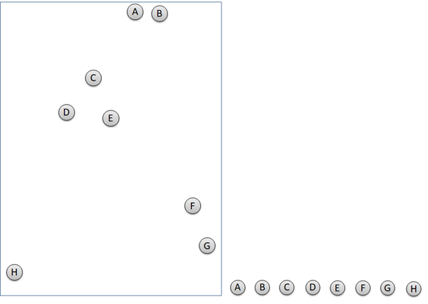
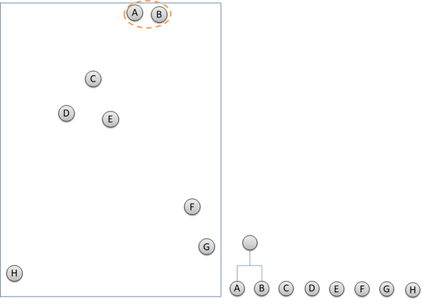
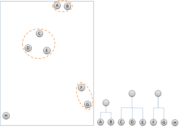
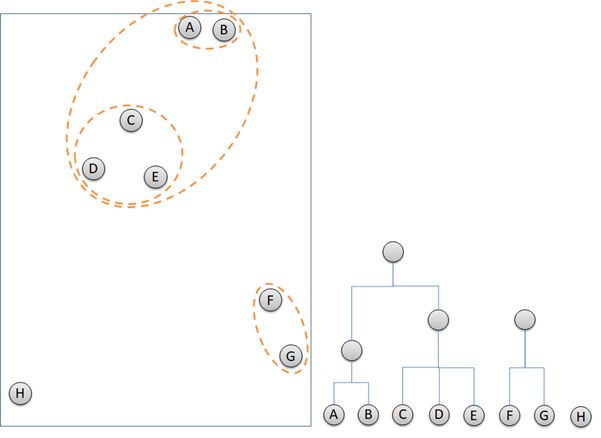
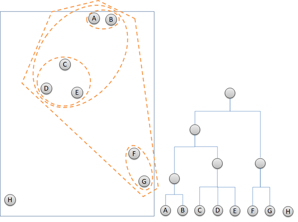
Hierarchical Clustering

Hierarchical clustering is an unsupervised machine learning that identify closest cluster and group them together. Basic of Machine Learning article can be found here. Hierarchical clustering works with only 2 steps repeatedly. Firstly, detect 2 or more closest points or clusters. Secondly, group them together. The next steps are the iteration of the first two steps until all of the data points are grouped in clusters. The illustration below describes how hierarchical clustering groups data points and build dendrogram at the same time.

Figure 2 Illustration of hierarchical clustering 2

Figure 3 Illustration of hierarchical clustering 3

Figure 4 Illustration of hierarchical clustering 4

Figure 5 Illustration of hierarchical clustering 5

Figure 6 Illustration of hierarchical clustering 6

Now, we will run the hierarchical clustering to a little bit more complex data, the Hotel Customer Data. ”. The data is dummy data I created. The data contains the information of customers opinion of a hotel. There are 500 observations or rows in this data frame. Each observation represents one customer. There are 12 variables, with data structure as following.

data.frame':   500 obs. of  12 variables:
 $ Id          : int  1 2 3 4 5 6 7 8 9 10 ...
 $ Gender      : Factor w/ 2 levels "Female","Male": 1 1 1 2 2 2 2 1 2 2 ...
 $ Age         : num  33 30 37 34 33 34 35 30 39 34 ...
 $ Purpose     : Factor w/ 2 levels "Business","Personal": 2 2 2 2 2 2 2 2 1 2 ...
 $ RoomType    : Factor w/ 3 levels "Double","Family",..: 1 2 3 1 1 1 1 2 1 1 ...
 $ Food        : num  21 32 46 72 84 67 56 10 73 97 ...
 $ Bed         : num  53 32 25 30 7 46 0 19 12 30 ...
 $ Bathroom    : num  24 18 29 15 43 16 0 1 62 26 ...
 $ Cleanness   : num  44 44 20 55 78 61 9 53 65 59 ...
 $ Service     : num  46 74 24 38 51 44 32 58 56 46 ...
 $ Satisfaction: Factor w/ 3 levels "Dissatisfied",..: 1 1 1 1 2 2 1 1 2 2 ...
 $ Repeat      : Factor w/ 2 levels "No","Repeat": 2 1 1 2 2 1 1 2 2 1 ...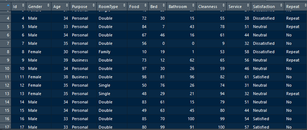

Customers are requested to fill a survey form to score 5 parameters of the hotel. The 5 parameters are food, bed, bathroom, cleanness, and service. The five parameters are scored in numeric from 0 to 100. 0 represents very bad and 100 represents very good. The objective of this article is to group the 500 observations in clusters according to the value of the five parameters.

# Scale the Customer data
Customer_scaled <- scale(CustomerData[6:10])

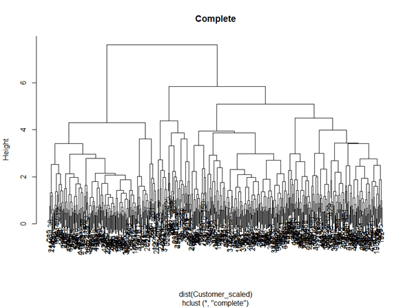
# Create hierarchical clustering model, using method = complete
Cluster_complete <- hclust(dist(Customer_scaled), method = "complete")

# Plot dendrogram 
plot(Cluster_complete, main = "Complete")

# suumarize the result
summary(Cluster_complete)

The script above firstly runs scale() to the parameters before build a hierarchical cluster. The scale() is to scale the parameters values to have mean of 0. This is to avoid to give more importance level to the parameters which have higher value than the others. There are some methods in the hierarchical clustering to determine the distance of one cluster to another. We will discuss this later. Now, we use the method = complete.

Figure 8 Dendrogram with “complete” method

# cut tree
# Cut by height
Cut_h4 <- cutree(Cluster_complete, h=  4.5)

# Cut by number of clusters
Cut_k4 <- cutree(Cluster_complete, k=  4)

Above is the dendrogram describing the clustering result. To simplify the dendrogram, there are 2 ways in cutting it. We can cut the dendrogram by the height or by the number of cluster we want. Below is to cut the dendrogram by the height 4.5, and to cut it to have only 4 clusters.

Figure 9 Cut tree at height 4.5 to have 4 clusters

Let’s visualize how the clusters look like.

# Plot the clusters
Customer_Cut_k4 <- data.frame(CustomerData, as.vector(Cut_k4))
names(Customer_Cut_k4)[13] <- "hclust"

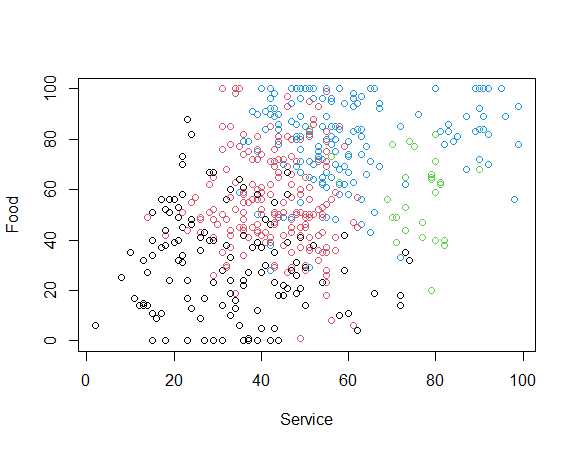
plot(CustomerData$Food ~ CustomerData$Service, col = Customer_Cut_k4$hclust,  xlab = "Service", ylab  = "Food", main = "Method = complete")

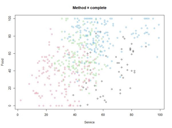
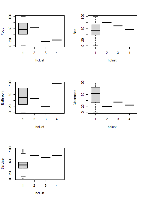
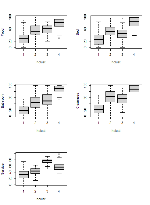
Unlike supervised learning, hierarchical clustering, as an unsupervised learning, does not have labels. So, we will need to analyze the clusters. Here is the data distribution.

# Analyse each cluster
par(mfrow = c(3, 2))

boxplot(Food ~ hclust, data = Customer_Cut_k4)
boxplot(Bed ~ hclust, data = Customer_Cut_k4)
boxplot(Bathroom ~ hclust, data = Customer_Cut_k4)
boxplot(Cleanness ~ hclust, data = Customer_Cut_k4)
boxplot(Service ~ hclust, data = Customer_Cut_k4)

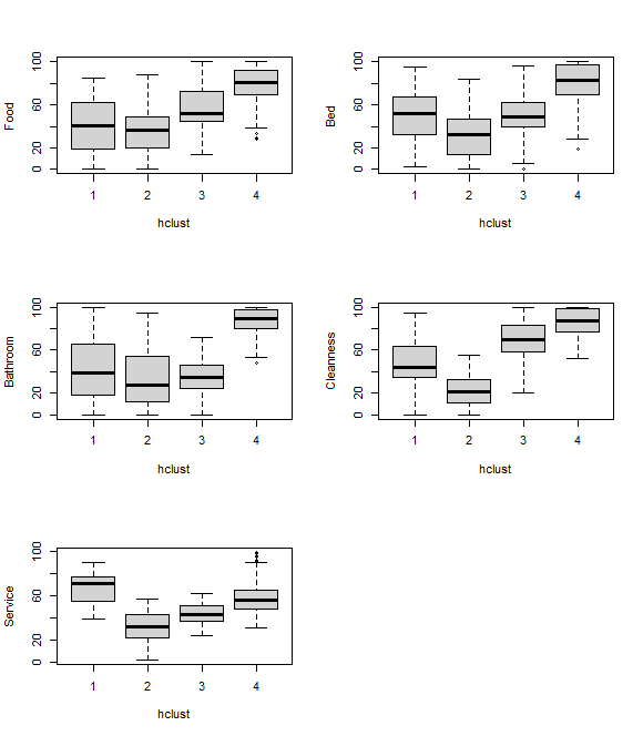
Customers in cluster 1 until 4 are distinguished by their data distribution of each parameter. Customers of cluster 4 had good impression to all of the parameters relative to other cluster customers. Customers of cluster 2 had worst opinion to the 5 parameters compared with other customers. Customers of cluster 1 were happy with the hotel service, but the other parameters were normal. Customer of cluster 3 had normal experience with all of the parameters.

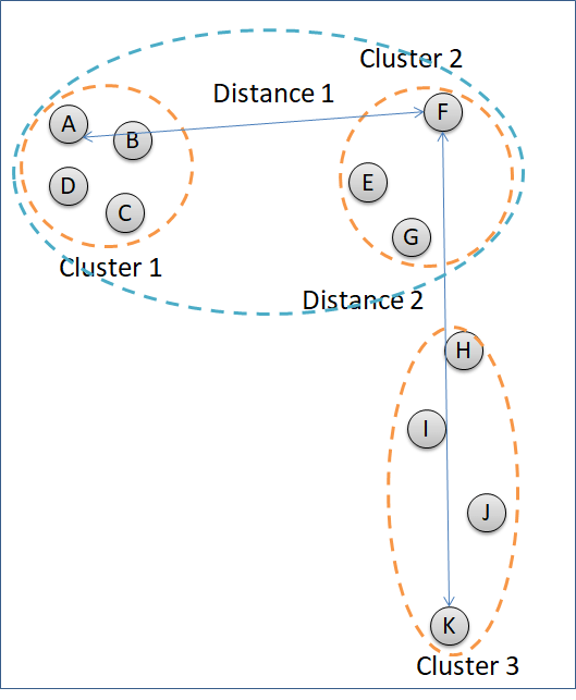
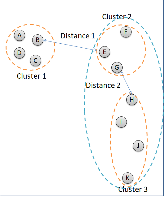
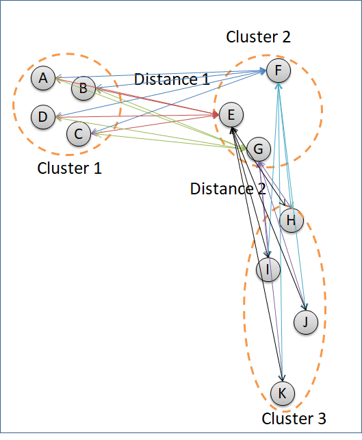
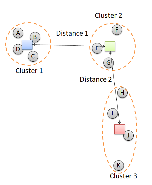
The example above uses the method = complete to cluster the data points. The method = complete groups clusters according to the least similar data points of the different clusters. In figure below, Cluster 2 is going to decide which cluster to combine with, Cluster 1 or Cluster 3. Distance of Cluster 1 and Cluster 2 is measured by point A and point F because the two points represent the least similar data points between the two clusters. Distance between Cluster 2 and Cluster 3 are calculated according to the distance of point F and point K. Cluster 2 will combine with Cluster 1 because the distance is shorter.

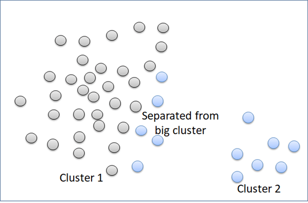
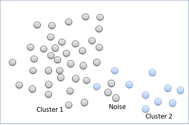
“Complete” method is good in clustering noise. But, it can break a big cluster.

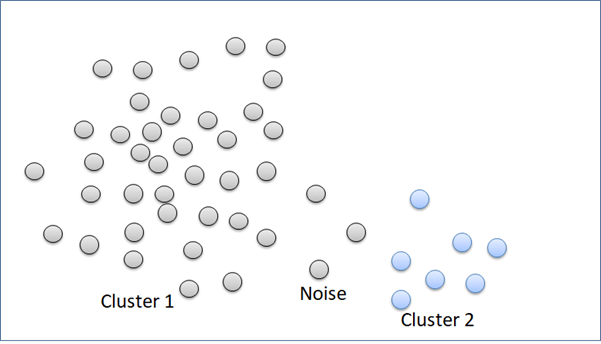
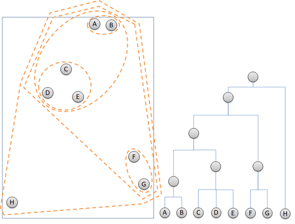
Figure 13 Clustering effectively among noise

The second linkage method in hierarchical clustering is “single”. This method groups clusters according to the most similar data points. In the picture below. Cluster 2 is grouped to the Cluster 3, instead of Cluster 1 because the distance of point G to point H is closer than distance between point E and point B.

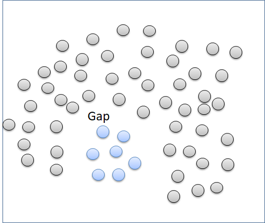
The “single” method can separate well clusters with a relatively big enough gap. The “single” method is not good in separating noise.

Hierarchical clustering using “single” method is performed using this script.

# Cluster linkage: single
Cluster_single <- hclust(dist(Customer_scaled), method = "single")

# Plot dendrogram 
plot(Cluster_single, main = "Single")

# Cut by number of clusters
Cut_k4_single <- cutree(Cluster_single, k=  4)

Customer_Cut_k4_single <- data.frame(CustomerData, as.vector(Cut_k4_single))
names(Customer_Cut_k4_single)[13] <- "hclust"

plot(CustomerData$Food ~ CustomerData$Service, col = Customer_Cut_k4_single$hclust,  xlab = "Service", ylab  = "Food")

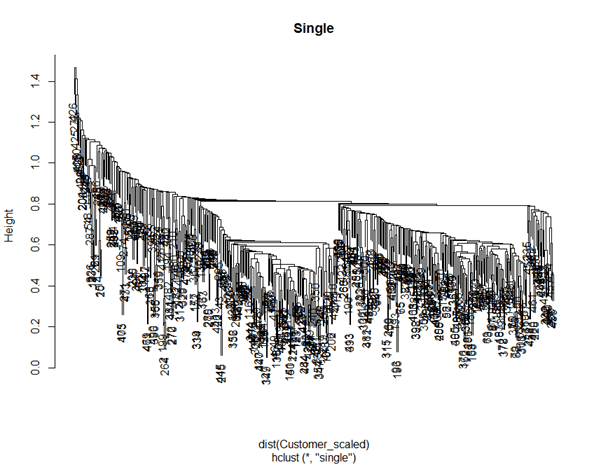
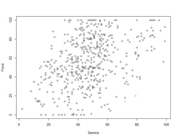
“Single” method described looks like not suitable for clustering CustomerData. “Average” method calculates the average distance of each data point of a cluster to each data point of another cluster before deciding which clusters have the shortest distance.

The script here applies “average” method to the hotel customer data.

# Cluster linkage: average
Cluster_average <- hclust(dist(Customer_scaled), method = "average")

# Plot dendrogram 
plot(Cluster_average, main = "Average")

# Cut by number of clusters
Cut_k4_average <- cutree(Cluster_average, k=  4)

# Analyse each cluster
Customer_Cut_k4_average <- data.frame(CustomerData, as.vector(Cut_k4_average))
names(Customer_Cut_k4_average)[13] <- "hclust"

plot(CustomerData$Food ~ CustomerData$Service, col = Customer_Cut_k4_average$hclust,  xlab = "Service", ylab  = "Food")