

Linear regression in a method in Machine Learning. The same term is also used in Statistics. To read about Machine Learning basic, please find my article here. Linear regression finds relationship between one or more continuous predictor variables and the dependent variable to predict. Simple linear regression has only one predictor or independent variable to predict the dependent variable. Plot the variables and draw a fit line with its distance to data points as small as possible. The distance of the fit line to each data point represents the prediction error.
Below is the data of 20 apples with their mass (gram) and volume (cm3). Now, we want to create a model or formula to estimate the volume of apple according to its mass using linear regression.
| Mass (g) | Volume (cm3) |
| 100 | 32 |
| 120 | 58.2 |
| 130 | 78.8 |
| 160 | 79.6 |
| 180 | 81.8 |
| 220 | 83.2 |
| 225 | 94.5 |
| 260 | 138.6 |
| 310 | 135.6 |
| 320 | 144.2 |
| 350 | 131 |
| 380 | 187.8 |
| 400 | 209 |
| 450 | 195 |
| 440 | 177.4 |
| 460 | 195.6 |
| 490 | 238.4 |
| 510 | 228.6 |
| 520 | 258.2 |
| 590 | 241.4 |
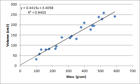
The model formula takes the form of y = mx + c where m is the slope (gradient) and c is intercept. The formula is Volume = (0.4415 x Mass) + 3.4058. Until here, you may think that this simple thing can be done easily using spreadsheet. Why need Data Science? It becomes more complicated if we have more than one predictors. Let’s try this Salary Data. This a data frame with 500 observations/rows and 5 variables. The variables are Id, Year of Experience, Level of Performance, Level of Responsibility, Salary. We will train a model using linear regression to estimate salary according to the 5 parameters.
The “Salary” is expressed in dollar. Year of experience “YearExp” is how many years the employees have experience. Level of performance “Performance” and level of responsibility “Responsibility” measure employees’ working performance and responsibility load. They range from 0 to 100.
> str(EmployeeData)
'data.frame':  500 obs. of  5 variables:
 $ Id            : int  1 2 3 4 5 6 7 8 9 10 ...
 $ YearExp       : num  23 15 10 5 21 10 1 13 6 7 ...
 $ Performance   : num  84 76 89 70 78 83 62 76 73 65 ...
 $ Responsibility: num  75 59 71 57 77 69 48 72 48 54 ...
 $ Salary        : num  7550 4609 5086 5860 5518 ...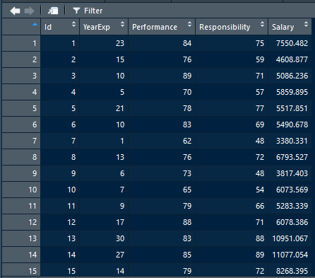

This script is to create the linear model
# Creating model
# Create linear regression model
linear_model <- lm(Salary~YearExp + Performance + Responsibility, EmployeeData)

# summarize the model
linear_model
summary(linear_model)
Here is the summary of the linear regression model. We can examine the residuals, coefficients, R squared, and others. Residuals show how different the predicted value to the actual value of the employee salary. The coefficients are used to make the linear regression. Salary = 715.888 + (YearExp * 109.000) + (Performance * 23.008) + (Responsibility * 30.153).
> summary(linear_model)

Call:
lm(formula = Salary ~ YearExp + Performance + Responsibility,
    data = EmployeeData)

Residuals:
    Min      1Q  Median      3Q     Max
-4196.4  -751.8   -31.3   849.6  4403.6

Coefficients:
               Estimate Std. Error t value Pr(>|t|)
(Intercept)     715.888    805.016   0.889  0.37428
YearExp         109.000     12.204   8.932  < 2e-16 ***
Performance      23.008     11.463   2.007  0.04528 *
Responsibility   30.153      9.858   3.059  0.00234 **
---
Signif. codes:  0 ‘***’ 0.001 ‘**’ 0.01 ‘*’ 0.05 ‘.’ 0.1 ‘ ’ 1

Residual standard error: 1404 on 496 degrees of freedom
Multiple R-squared:  0.5926,   Adjusted R-squared:  0.5901
F-statistic: 240.5 on 3 and 496 DF,  p-value: < 2.2e-16
The following script predicts the salary values using the linear regression model and plot them in ggplot.
# predict the salary according to the linear model
prediction_Linear <- predict(linear_model, EmployeeData)
prediction_Linear <- data.frame(EmployeeData, prediction_Linear)

# plot the actual vs predicted salary
ggplot(prediction_Linear, aes(x=Salary, y= prediction_Linear)) +
  geom_point(alpha = 0.3) +
  geom_abline(color = "blue")

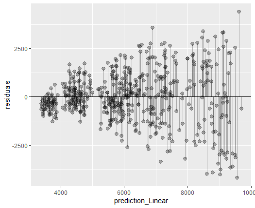
After we get the model, now we want to evaluate the model. We want to evaluate how far the predicted values from the model are from the actual values. Below plots the residuals of the model. The farther the points from the horizontal line suggest the farther the predicted values from the actual values.
# Evaluating model
# Visualize residuals

# Compute residuals
prediction_Linear$residuals <- prediction_Linear$Salary - prediction_Linear$prediction_Linear

# Fill in the blanks to plot predictions (on x-axis) versus the residuals
ggplot(prediction_Linear, aes(x = prediction_Linear, y = residuals)) +
  geom_pointrange(aes(ymin = 0, ymax = residuals), alpha = 0.3) +
  geom_hline(yintercept = 0, linetype = 1)
Besides graphically, model evaluation can be done by the Root Mean Square Error (RMSE) and R-squared.
> # RMSE
> (rmse_Employee <- rmse(prediction_Linear$Salary, prediction_Linear$prediction))
[1] 1398.215
>
> # standard deviation. If RMSE < SD, it is good
> (sd_Employee <- sd(prediction_Linear$Salary))
[1] 2192.819
> # Get the correlation between actual and predicted data
> (correlation <- cor(prediction_Linear$Salary, prediction_Linear$prediction_Linear))
[1] 0.7698109
The RMSE is 1398.215 and the standard deviation is 2192.819. If the RMSE is higher than the standard deviation, the model is not good enough. The R-squared is 0.5926. It is shown above in summary(linear_model). The correlation between predicted and actual values is 0.7698.
There is an evaluation method named split test. The EmployeeData is split into 2. The 500 rows are split into 100 and 400 separated data. Each of the split data will be used to create a linear model. After the two linear models are created, prediction and evaluation are run again to get the 2 values of RMSE and the 2 values of R-squared from the two split data. The RMSE and R-squared values should be similar to say that the model is good.
# Split test
# create 100 sample
sampleIndex3 <- sample(1:500, 100 , replace = FALSE)

# split the EmployeeData into 400 and 100
Employee_split1 <- EmployeeData[sampleIndex3,]
Employee_split2 <- EmployeeData[-sampleIndex3,]

# predict salary of test data
Employee_split1$prediction <- predict(linear_model, Employee_split1)

# predict salary of training data
Employee_split2$prediction <- predict(linear_model, Employee_split2)
> Compute both RMSE and compare if they are close
> (rmse_split1 <- rmse(Employee_split1$Salary, Employee_split1$prediction))
[1] 1360.313
> (rmse_split2 <- rmse(Employee_split2$Salary, Employee_split2$prediction))
[1] 1407.531
>
> # Evaluate the r-squared on both training and test data.and print them
> (r2_split1 <- (cor(Employee_split1$Salary, Employee_split1$prediction))^2)
[1] 0.6111988
> (r2_split2 <- (cor(Employee_split2$Salary, Employee_split2$prediction))^2)
[1] 0.5878237
1 thought on “Linear Regression (Supervised Machine Learning)”